Population modeling with dynamic models

One of the most important questions in ecology is how populations of animals grow and decline. This turns out to be a very hard question. There are many population models, but so far none of them can be considered a final answer.

Population models can be simple or complex, but they are all dynamic models. A dynamic model includes time as a dependent variable. A dynamic model run involves starting the variables off at some initial values, and then calculating how the variables would change over time according to the equations of the model.

The figure at left shows the results of one run of a dynamic model for the number of yeast cells in a fermentation vat, The graph shows a single variable, which is the number of yeast cells. The initial value was chosen as 1000 yeast cells. Over time the value increases to about 2700 and then “crashes” toward the right side of the graph. We will discuss the structure of this model later in this chapter.

This type of model is fundamentally different from the linear models we have considered in the previous chapter. In the linear model, you give each input variable a value, and then “turn the crank” one time to get the resulting output value. In a dynamic model, here is what you do:

1. Set the time variable to zero and the other variables to their chosen initial values;

2. “Turn the crank” to get the values of the variables at some time shortly after the start. In the yeast example we compute the population after one day.

3. Repeatedly “turn the crank” to calculate the values for two days after the start, three days after the start, and so on.

This calculation process is called simulation. In this chapter we will crank up some dynamic models using Microsoft Excel and Stella. But first, we need to define a few important terms.

Population, growth, and growth rate

Suppose you hear that the population of suburban Glitter County, Georgia rose from 185,000 in the year 2000 to 188,400 a year later. Meanwhile, the population of rural Boondock County rose from 13,400 in 2000 to 14,200 in 2001. Which county is growing faster?

he answer depends on what you mean by “growth.” There are two terms that are commonly used to define growth:

· Growth simply means the difference we get by subtracting the old population value from the new one. For example, we find the population increase for Glitter County by subtracting 185,000 (the 2000 population) from 188,400 (the 2001 population). We find that Glitter County’s population growth was 3,400 people in one year. This measure is also called the absolute growth.

· Growth rate is defined as the growth divided by the old population. This simple definition only works if the time period between the old and new is one year, or one month, or one time unit of some sort. Growth rates are expressed as percents and include a time unit. For example, the growth rate of Glitter County is 3,400 divided by 188,000. This works out to about 0.01837. We express this by saying Glitter County had a growth rate of1.8% per year.

With these definitions in mind we can compare the growth and growth rate for Glitter County and Boondock County.

	Glitter County	Boondock County
2000 Population	185,000	13,400
Population growth 2000 – 2001	3,400	800
Population growth rate 2000-2001	1.8%	6.0%

Table 1. Population growth vs. growth rate for two counties.

From the table we can see that Glitter County’s absolute growth was larger, but Boondock County had the higher growth rate. Boondock’s 800 new residents are a much higher percentage of its existing population than Glitter’s 3,400 new residents. It is likely that Boondock County will experience more of the stresses caused by population growth, such as congested streets and overcrowded schools.

Another way of expressing the relationship between absolute growth and growth rate is this:

· The absolute growth equals the growth rate multiplied by the initial population.

You can test this out by multiplication in the table above. For Glitter County, multiplying 1.8% by the initial population of 185,000 will give you approximately 3,400. For Boondock County, multiplying 6% by the initial population of 13,400 will give you approximately 800.

Linear and exponential growth

In real life, we usually do not have yearly figures for the population of a county. Instead, the census gives us a population figure every ten years, in 1990, 2000, etc. What would we do if we wanted to estimate the county’s population in, say, 1994?

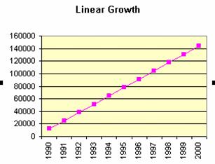
One way to estimate the 1994 population is to assume that the county had the same absolute growth in each of the years 1990 through 1999. Under this assumption the graph of population size looks like Figure 2. The 1994 population from this graph is 64,800.

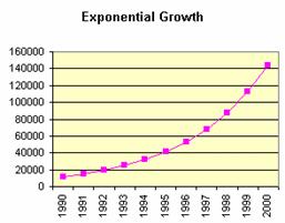
Another method would be to assume the county had the same growth rate in each of the years 1990 through 1994. Under this assumption the graph of population size looks like Figure 3. The 1994 population from this graph is 32,423 – quite a bit lower than in the first case.

Let’s take a moment to examine these two graphs. Each graph starts with a population of 12,000 in 1990 and increases to 144,000 in 2000.

In Figure 2, the absolute growth is 13,200 people each year. Having the same absolute growth each year makes the graph a straight line. This pattern of growth is called linear growth.

In Figure 3, the absolute growth is increasing each year. The percentage growth is constant at 28% per year, every year. But each year we take 28% of a larger base population. In 1990, the absolute growth is 28% of the original 12,000 people. This multiplies out to 3385 additional people. By 1999, the population has grown to 112,316. Multiplying 28% by this number gives us an absolute growth of 24,712 people for 1999.

This pattern of growth, in which the growth rate remains constant, is called exponential growth. The upward curving shape of the graph in Figure 3 is a characteristic of exponential growth.

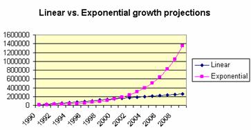
Exponential growth is important because, if it continues for any length of time, the population will grow dramatically. We can illustrate this by projecting the future growth of this population using the linear growth pattern and the exponential growth pattern. The results of this calculation are shown in Figure 4.

If you compare Figure 4 with Figures 2 and 3 you will notice that the Y-axis scale is very different. The graphs in Figures 2 and 3 are both scrunched into the bottom of Figure 4. You can just barely see that the two curves are equal in 1990 and in 2000, and that the exponential curve is underneath the linear curve between 1990 and 2000.

In both curves the population continues to grow after 2000. The linear curve increases to 262,000 in 2010. This is almost double the 2000 population – a big increase. But the exponential curve increases to 1,374,000, which is 12 times the 2000 population! The term population explosion is used to describe a period of continued exponential growth.

Calculating exponential growth using Excel

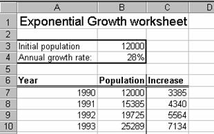
In Figure 5 you can see the first few rows of an Excel worksheet. This calculation was used to create the graph in Figure 3.

To create worksheets like this, we must first identify the key variables in the model. In this case they are the year, the population in that year, and the population growth in that year.

Once we identify the variables, then we use a separate Excel column for each variable. Our worksheet will be much easier to understand if we give an appropriate label to each column. You can see these labels in row 6 of the worksheet.

It also is very helpful to identify the key parameters of the model. A parameter is a number that is important to the model, but does not change as a variable does. In this case the annual growth rate, 28%, is a parameter. The initial population size is also a parameter. We create a box to hold the parameters and explain their meaning.

All the rest of the numbers in this model are calculated based on these two key parameters. To experiment with the model, we would simply change the values in cells B3 and B4. Excel will automatically re-compute the rest of the numbers and re-draw the charts.

Finally we need to write the formulas which make up columns B and C of the table. This is not hard, as long as we first express in English what the formulas are supposed to mean. Then, we can translate the English statements to algebraic formulas.

Cell	Meaning of result	How to calculate result	Formula
B7	1990 population	Same as “initial” population	=B3
C7	1990 absolute growth	28% of current population	=B7*$B$4
B8	1991 population	1990 population plus growth	=B7+C7
C8	1991 absolute growth	28% of current population	=B8*$B$4

Table 1. Calculations for the first two rows of the exponential growth table.

Pay particular attention to the formulas for cells C7 and C8, the second and fourth rows of Table 1.

· Both formulas contain references to B4, which contains the growth rate 28%.

· The part of the formula that represents the current population is different between the two formulas.

The dollar signs in these two formulas are Excel absolute cell references. They do not affect the calculated result of the formula. But when we copy the formula, Excel will not change the absolute references. This allows us to finish the table by copying the two formulas in cells B8 and C8 to the rest of the rows in the table! Consult your Excel lab manual for more information and examples about cell references and copying formulas.

The most important part of Table 1 is not the last column. It is the third column, which contains the English explanation of how to compute the results. Many students skip this part of the process, and try to write down the formulas without being able to explain what they mean. Usually, the formulas will end up being wrong because we don’t understand their meaning.

These students typically complain that they cannot create the worksheet due to their poor math skills. In reality, their English skills are more important! If you take the time to say in English what is going on, you will find it much easier to compose the Excel formulas to carry out your calculations.

Calculating exponential growth using Stella

We can use the Stella modeling program to create a graphical version of the exponential growth model. As with Excel, there are three variables:

· The time

· The absolute growth

· The population size

Recall that the growth rate and initial population size are parameters, not variables. That is, the growth rate and initial population size do not change during the model run.

One difference in how we set up the model is that Stella automatically creates the time variable for us. So we need only to define the growth rate, absolute growth, and population size.

Exponential growth and doubling time

Exponential growth occurs whenever some quantity increases at a fixed percentage rate per year. Population is one quantity that sometimes behaves this way. Another is money in a bank.

Suppose you deposit $100 in a bank account that pays 4% interest per year. That means that after a year, the bank adds $4 in interest and your account balance is now $104.* Now suppose you ‘let the money ride’ for another year. Then the bank will pay interest again. This time they will pay 4% of $104, or 4.16. Your account balance will now increase to $108.14. Yippee!

In other words, your money in this bank will increase by 4% every year. The fact of a constant percentage growth rate is enough to guarantee exponential growth. The same Excel worksheet or Stella model used above will also calculate your bank balance. In modeling we say,

· The same problems have the same solution.

This means that problems with the same mathematical structure have the same solutions, even if the real-world context is different. A growing caribou herd looks and smells a lot different from a Certificate of Deposit at your local bank. But to a modeler, the two situations are no different – they are both examples of exponential growth.

How long would it take for your account to double, to $200? We could answer this question by running the Excel or Stella model. But there is an easier way. For any quantity which increases by a constant percent per year,

· Doubling time = 69 / (percentage rate of growth)

A bank account that pays 4% interest, or a caribou herd that increases at a rate of 4% per year, will each double in about 69/4 or 18.25 years.

Exponential growth in the US economy

Another quantity that grows exponentially is the overall size of the US economy. Actually the economy doesn’t quite grow exponentially, because the growth rate changes from time to time. When the growth rate is under about 2 percent a year, people talk about a “slumping economy.” When the growth rate rises to over 4 percent or so, people talk about a “booming economy.”

In the long term, the economy looks more like a classical exponential curve, with a growth rate of about 3 percent a year during the 1900’s.

Almost everyone prefers a booming economy, except environmentalists who worry about the ecological consequences of all this growth. We will have more to say about this in a later chapter.

Growth in a limited environment

You don’t need a Ph.D. in ecology to figure out that the exponential growth model cannot describe real populations over the long term. If a population keeps doubling over and over again, it must eventually overflow the capacity of its environment to sustain it.

Understanding the actual increases and decreases of animal populations is very hard. However, it’s easy to make a model that includes the effect of a limited environment.

Ecologists define the carrying capacity of a given environment as the maximum number of animals the environment can support over a long period of time. For example, the carrying capacity of the Arctic National Wildlife Refuge to support caribou is determined by the amount of grass and lichen growing on the tundra there. If we somehow put in a herd of caribou that was much larger than the carrying capacity, they would overgraze their habitat and an ecological disaster might result.

To use the carrying capacity in a population model, first think about what the population growth curve should look like. Suppose that we start with a herd of caribou that is much smaller than the carrying capacity. These “pioneer” caribou will perceive an environment that is practically infinite. This means that any limits to growth would have a negligible effect. We would expect that

· When population size is small, growth is nearly exponential.

The situation will be very different when the population gets close to the carrying capacity. Shortages of food and other resources would slow down the increase of the population. If population actually reaches the carrying capacity, it should not increase at all.

· As population approaches the carrying capacity, growth slows down.

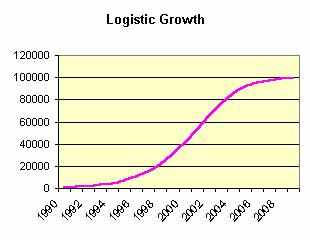Taking these two points into consideration, what we want is a population curve that looks like Figure 7. In the left half of this graph the population follows an upward-sloping curve, similar to an exponential curve. But in the right half of the graph the population levels off to its carrying capacity, which is 100,000 in this case. Ecologists call this growth pattern logistic growth.

How do we change the exponential model to create this behavior? The first step in model definition is to decide on the model variables.

Remember that variables are key numbers that change during a model run, while parameters are key numbers that do not change. In the exponential model, growth rate was constant. But in the logistic model, growth rate starts out at a high level and gradually declines as the population approaches its carrying capacity. So we must make two changes to the exponential model:

· Growth rate becomes a variable instead of a parameter.

· A new parameter, carrying capacity, must be added.

Modeling logistic growth in Excel and Stella

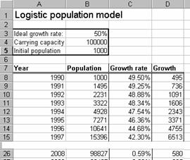A new Excel worksheet that reflects these changes is shown in Figure 8. Note that there is now a new column for growth rate, which has become a variable.

Also note that there is a new parameter called “ideal growth rate.” This represents the growth rate that would hold if there were no environmental constraints at all. If you examine column C in Figure 8, you will see that the actual growth rate variable starts out very close to the ideal value, and gradually declines over time.

How do we actually calculate the growth rate in column C? Ecologists looking for a simple model came up with the following equation:

· Actual growth rate = Ideal growth rate * (1 – Population / Carrying Capacity)

This equation has the desired behavior which ecologists want:

· When population is very small compared to carrying capacity, the expression in parentheses evaluates to almost 1. In this case the actual growth rate will be close to the ideal growth rate.

· When population is close to the carrying capacity, the expression in parentheses evaluates to close to zero. In this case the actual growth rate will be close to zero as well.

It is important to understand that this equation was ‘cooked up’ to produce the kind of model behavior that the ecologists wanted. Whether actual populations ever behave like this is a matter for field studies.

Figure 9 shows how to revise our Stella model to calculate logistic growth instead of exponential growth. As in the Excel case, we have added “ideal growth rate” and “carrying capacity” to the model.

Figure 9: Stella logistic model.

Both of these new concepts are considered converters in Stella parlance Converters don’t represent actual population, or flows of population. They are concepts that control population flow, as shown by the arrows leading into the big valve icon. Note that some converters can control other converters.

Positive and negative feedback

The exponential and logistic models illustrate two key ideas in the study of dynamic systems.

· A positive feedback loop reinforces changes in a variable;

· A negative feedback loop diminishes changes in a variable.

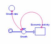Positive feedback loops are also called “self-stoking cycles.” The virtuous cycle of mainstream economic theory is a good example. A bigger economy generates more growth, which makes the economy bigger, which generates more growth, etc. etc.

A similar positive feedback loop drives the population models. A higher population creates a bigger annual increase, which makes the population bigger, etc. etc.

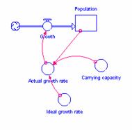
The logistic population model also has a negative feedback loop between population and growth rate. Just that 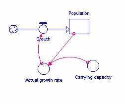part of the Stella model is shown in Figure 11. A higher population creates a smaller actual growth rate, which in turn creates a smaller annual population increase. The result is not to reduce population, just to slow its increase.

The classic example of negative feedback is your house thermostat. If the house gets colder than desired, the thermostat turns on the heat. If the house gets too warm, the thermostat turns off the heat. As a result, the house temperature will stay near the desired value.

Positive feedback in a model tends to create accelerating growth, while negative feedback tends to maintain the model in a steady state. The two types of feedback are like the accelerator and the brake pedal in a car.

Harvesting and maximum sustainable yield

Many animal and plant populations are also important economic resources. Fish populations such as cod, the Atlantic bluefin tuna, and many others are examples. In recent years overfishing has threatened many of the world’s most important fisheries with collapse.[1] Governmental agencies and international commissions use population modeling to manage, and hopefully preserve, these fish stocks.

We can extend our logistic population model to include the effects of harvesting. The basic equation will now be

· New population = Old population + natural growth – harvested amount

This equation says that if a fish population’s natural growth is more than the amount of fish caught each year, the population will continue to increase. But if we harvest more fish than the natural growth, the population will decline. If we harvest precisely the same amount of fish as the population’s natural growth, then the population will be constant. In theory, we could continue to harvest this amount of fish each year forever.

The ideal situation from an economic point of view is to harvest the same amount of fish each year, and make this amount be as large as possible without causing the fishery to collapse. This strategy is called maximum sustainable yield.

We can discover the maximum sustainable yield by examining the natural growth variable in the logistic model. (We assume the model now represents tons of bluefin tuna, not people!) In Figure 12 we have selected the year with the largest growth, and drawn a vertical line in the population graph at this point.

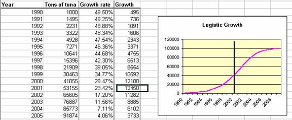
Figure 12. Maximum natural growth occurs at about half the carrying capacity.

You can see from the chart in Figure 12 that the maximum natural growth is also the steepest point on the population curve. This is also the theoretical maximum sustainable yield.

Now we can add a variable named Harvest to our model. In order to harvest a population at its maximum sustainable yield, we must wait until the population has reached its maximum natural growth. Can you see why? In this model, let’s wait until 2004 to begin harvesting the tuna population. The resulting model will look like Figure 13:

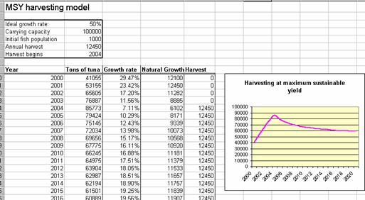
Figure 13. Harvesting at maximum sustainable yield (MSY) starting in 2004

Please examine the first few rows of Figure 13. (We have hidden the 1990 – 2000 period to make the picture simpler). The natural growth reaches 12,450 tons in 2001. Between 2001 and 2004 the natural growth slows down because the fish population is approaching its carrying capacity.

Starting in 2004, the harvest is more than the natural growth. This makes the fish population go down. But because the fish population is close to the carrying capacity, reducing the fish population makes its growth rate go up! This negative feedback has the effect of stabilizing the system. As you can see in the chart in Figure 13, the fish population begins to level out. This level of fish will allow 12,450 tons of fish to be harvested every year indefinitely. In other words, the fishery is being sustainably harvested. International fishing bodies establish fishing quotas to enforce these limits.

The model also shows us what can go wrong. Suppose that through cheating or honest error, fishers harvest more than the maximum sustainable yield of fish each year. The grim results are shown in Figure 14.

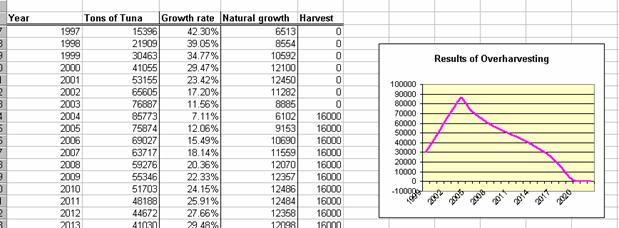
Figure 14. An unsustainable rate of harvesting leads to fishery collapse.

In figure 14 we see that once the fish population is below the MSY level, decreasing the population makes the natural growth go down. This positive feedback loop destabilizes the population, leading to collapse. Positive feedback is not necessarily good!

Delayed feedback and stability

The logistic model gives a very clean result, in which population size settles smoothly in on the carrying capacity of the environment. However, this model makes an important assumption that may not describe actual populations:

· In the logistic model, the population growth rate decreases without delay as the population approaches its carrying capacity.

In real populations, there may be a delay before the population reacts to approaching its carrying capacity. For example, a herd of reindeer may be overgrazing its land, but it is incapable of recognizing this fact and controlling its population growth. The result is a tragic overshoot and collapse scenario. The population not only declines, but the carrying capacity is decreased – the degraded land can no longer support the same number of reindeer.

Chapter review questions

1. A bank account pays 7% interest. How many years will it take for money in this account to double?

2. An experimental population of bacteria doubles in size every 8 hours. What is the growth rate of this population? (The answer will be some number of percent per hour, not per year.)

3. The explanation of how a house thermostat works assumes that it is winter, when the furnace is on. Restate this explanation for the case when it is summer and the air conditioning is turned on.

4.

---

* Actual banking practice is a great deal more complicated than this, but the basic idea is the same and the results will be similar.

[1] Tom Athanasiou, Divided Planet: the Ecology of Rich and Poor, pp. 69-70 University of Georgia Press, 1996.