
Assignment 2: Diving into Excel : Heads or Tail?
Q1-Q3 complete below. Q4 and Q4 is due Wednesday and is not complete (yet)!
| Assignment Day | Friday, August 23, 2013 |
| Due Date (Data) | Friday, August 23 |
| Due Date (the Q2-Q3) | Monday, August 26, 2013 (midnight - the midnight that is after Monday's class) |
| Due Date (the Q4-Q5) | Wednesday, August 28, 2013 (midnight after W Class). |
| Format | Class Email List (Data), ELC (the Rest - maria@cs.uga.edu) |
-
Send a message to the mailing list with your excel sheet for the tosses. {Due Today}
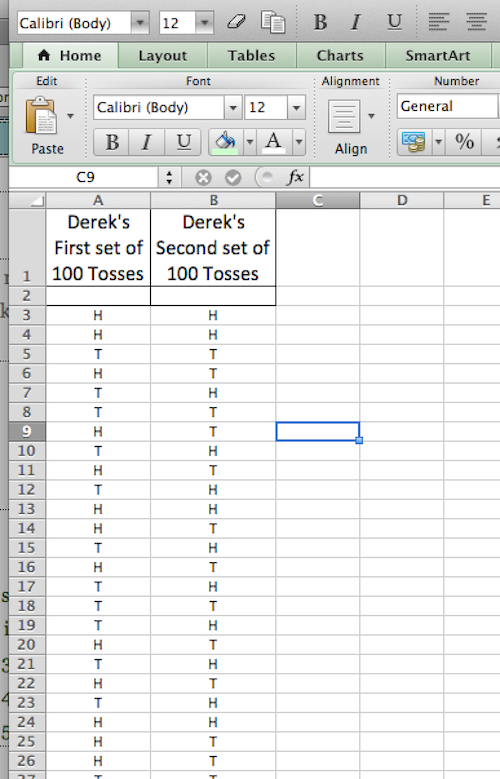
Example: here (Derek's tosses in an excel file). Note: if your 200 tosses are all in Column A, that is OK.
Figure Q1: Example spreadsheet for Question 1 and Question 2.
.
- For this question you will need to recreate the excel that we did in class Monday (the goal is to introduce you to the IF function).
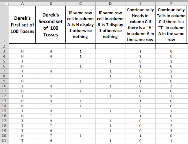
Step I: Create a new workbook, save it as YOURLASTNAME.xlsx. Example: I would save mine as, Hybinette.xlsx. In this new workbook, paste into Column A, starting at Row 3 (as Derek's file in Figure Q1 (above), the result of your first 100 tosses. [Copy : by menus File->Copy OR by keyboard Ctrl-C for windows and Command-C for macs || Paste : by menus File->Paste OR by keyboard Ctrl-V for windows and Command-V for macs, after copying, you paste by putting the mouse where you want the sequence to start - so put the mouse in cell A3]. Also paste into Column B, the result of the last 100 tosses of your experiment using similar techniques that you used for the first 100 tosses.
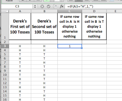
Step II: In this step you will continue filling in column C and column D. Column C cells should display a 1, if the corresponding cell in A (the cell that is in the same row of the cell in column C) is an "H", and it should display nothing (an empty string) if the cell is a "T" (see figure below). To attack this, you should start by typing a forumula in one cell, lets say we will type in cell C3. In class we used the IF function to display 1 when H was in column A.
Figure: Q1-StepIIa:
 ''
''
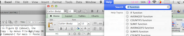
You can find out details on how the IF function work by typing "IF function" under the right most Menu HELP. See how to get help on an excel topic using help in the image below. The IF function should test whether the cell in column A that is in the same row as C is a H, if it is it should display a 1, otherwise the empty string ""). HINT: make sure to put double quotes around H, i.e, "H" in the IF formula for heads.
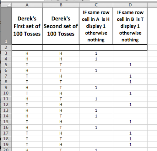
Now after you typed in the formula in Cell C3 (as depicted in Figure: Q1-StepIIa), you will need to fill in the rest of the cells in column C. You do this by using the fill handle. This is done by selecting the cell in C3 with your mouse, then you pull the lower right blue box down to row 102 (or the last row that contains data in column A). While doing this be sure only to target column C. Now the formula is copied to the other cells in column C so that they display a 1, if cell in A is a head. You should repeat this steps for for column D, but insteasd of testing for heads in column A, you will need to test for tails in column A.
Your result should look like something like the below image (Figure A1-StepIIc). Of-course it will not be exactly the same, since your tosses are probalby not exactly the same as Derek's tosses.
Figure: Q1-StepIIc:
- Step III: For this question you will need to recreate what we did in class Wednesday. The goal now is to figure out a process on how to count occurences of a specific length of a sequence. for example in the immediate image above Column A contains 18 tosses, these particular tosses contains the following sequences of 2 (HH (row 3,4), TT (row 7,8), HH (row 13, 14)), so 3 sequence of length 2. It contains 1 sequence of length 3 (row 17, 18, 19 of Tails).
We could do this by keep a tally of head and tails in 2 separate collumns, and we could increment our tally by one from the cell above, if we see a head in the current row. So, to get started, lets say we are tallying the heads in column E (see image below). The cell in A in row 3, shows an H, so when we are in row 3, in E we would put a 1 for our tally in E3. When we tally heads in row 4 in E, we notice that we tossed a head again in A, so we should increase the tally by 1 in row 4. When we continue to row 5 in E, we see that we tossed a Tail (T), so we should reset the tally to 0 and display a 0. The result of tallying heads in E should look like the image below, for tosses in column A.
We should uset he IF formula again, so =IF(logical test , do this if value of test is true, do this if value of test is false). So if has 3 parameters.
IF we write our formula in cell E3, we should test the cell in A3 for the character "H", so A3="H", for the test/ or condition. Now if the value is true, i.e., if A3 is an H, then we should look a the cell above us in column E, and then increment that value by 1. Since we are in cell E3, the cell above is E2, so this parameter should be E2+1. Note that,this is our first toss, so E2 in the image below is "", so we may want to intialize the tally by entering a zero in E2 (same for F2).
The third parameter of IF, denotes what we do if the condition of the test is false. For example, when we tally the value of A5, we note that we tossed a tail. Since it is a tail we should not tally this toss, and reset out counter or tally to 0.
Once you finished typing the =IF formula in E3, you should fill in the rest of the cells by dragging the fill handle down, similarly to what we did in step 2. You should also use a similar Logic and tally Tails in Column F. In Summary for column E (tallying heads)
1) Use the =IF formula in E3
2) Fill in the 3 parameters in the IF Formula = IF( paramater 1, parameter 2, parameter 3)
3) Parameter 1: test whether there is tail in A3, i.e., A3="H"
4) Parameter 2: type what to display if A3 is a head, so, increment cell above (E2), by 1, so E2+1
5) Parameter 3: type what to dipsplay if A3 is NOT a had, so 0.
6) Use the fill handle for the rest of the column. (check whether it filled in correclty by inspection)
Repeat this logic for column F (but now tally tails).
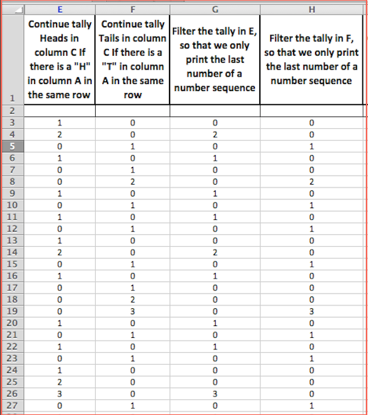
Step 4: Now we need to filter the result of the tally so that we only display the last number of an the increasing number sequence, for example, suppose we have the sequence 0000123401230 (going down a column), there are two increasing number sequences 1234 and 123. Here we should only display the last number of the tally of each increasing sequence before they resets to 0 again. The first sequence is of length 4, and the second sequence is of length 3, and for the next column we would like to display the sequence 000000040003 (4 is the last number in the first sequence, and 3 is the last number in the second sequence). Note that from this new column, we can easily spot that there is one sequence of heads that are of length one, and there is another sequence of length 3.
As another example, in Derek's data (see below) column F, we see that Tails, have the following sequences: 7 sequences of tails of length 1 (F5, F10, F12, F15, F21, F23, F27). Note, the last one, F27, maybe of a different size, since we don't see a terminating 0), so we should probably say 6 sequences of length 1. There is one sequence of tails of length 2 (F7, F8), and there is 1 sequence of size 3 (F17, F18, and F19). In column H we see that we have filtered column F's result by only displaying the largest number of each sequence. Not that in H it is much simpler to spot how long, and the frequence of each length sequences. We can quickly spot that there is only one sequence of length 2, and one sequence of length 3.
We can do this by using a combination of 2 functions in excel, IF and AND. AND returns true if two conditions are TRUE, and FALSE otherwise. Please use the help menu in excel for further details.
Lets consider that we are the last head in a sequence of heads, and lets suppose we are currently
evaluating what to do (print) for cell G4. We notice that in E4 we are tossing the last head in a sequence of length 2 of heads. The cell below E4 (i.e., E5) is a zero, indicating we tossed a tail, therefore terminating the sequence of heads. So we are looking at the cell below the row that we are evaluating to determine if we are at the end of a sequence AND we are checking whether we are still tossing a head (i.e, by evaluating the same row cell in E as G4, i.e., E4. So two conditions need to be true to determine if we print a number.
BOTH the below conditions need to be TRUE:
* E4 is not 0 translates to E4 <> 0, and
* E5 is 0, E5=0
So we should use AND to evaluate two conditions that are true simultanoulsy witing an IF statement.
=IF( AND( condition1, condition2 ), what do if AND is true, what do if AND is false )
We should print E4 in G4 if and is true, and 0 (zero) otherwise.
Fill out the rest of column G by using the fill handle, and also filter the tally of tails in column H, your result should have the same effect as the below image.
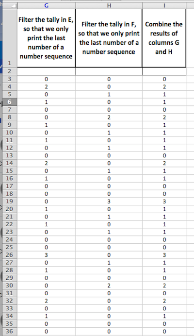
Step 5: Our next is to combine the results of column G and H into a single column, column I. The goal is to display all lengths sequences in one column, independent whether they are heads or tail. To make it more clear lets look at column G and H and we will focus on rows 3-9 (7 tosses HHTHTTH, the next toss is a T (row 10). G displays 0201001, and H displays 0010020.
Lets describe the sequence of heads and tails: We see a sequence of length 2 of heads, then we see a sequence of length 1 of tails, then there is a sequence of length 1 of heads, then there is a sequence of length 2 of tails, and finally there is a sequence of length 1 of heads. We can generate this 'verbal' sequence as: 0211021 (we use 0, when we are still running a sequence, so the first toss we are still tossing Heads, so we use a zero for the first toss since we are "not done" tossing heads.
We can combine G and H easily by noting that we only need to keep track of the largest value of the value of the cell in G or H. Thought question (Why?). To display the largest value of two cell values we can use the function =MAX(a list of cell values).Check out MAX() function using HELP. In cell I3, type =MAX(G3,H3). Then fill the rest of the column byusing the fill handle. See the figure below what the result should look like.
- Step 6: Frequency (Q4/Q5 will be due Friday after class).
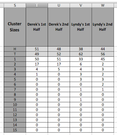
For this exercise we will count the frequency of each length sequences. For example in Derek's first 100 tosses we like to see how many sequences that are of length 1, and how many sequences that are of lenght 2, and so on. By looking at our column Ifrom the previous exercise above we could just count each length sequences by inspection. For example by looking at rows 3-36, we see that there are at 2 sequences of length 3 by counting the occurences the number 3. And we can count the occurences of sequences of lenght 2 by counting how many times the number 2 occurs in column I. Of-course if we count all 100 tosses, we should expect that there are more occurences of each of these lenght sequences. In fact there are 17 sequence of size 2, 4 sequences of size / lenght 3 and 1 sequence of length 4.
From this data we can create a frequence table see below figure. The occurences of each sequuence is under the column titled "Cluster Sizes" below. Cluster size is simly the frequence of different lengths of tosses.
How can we create this frequence table in Excel? The first step is to use the function: =COUNTIF function. COUNTIF has two parameters, a range and a criteria.
=COUNTIF( range, criteria )
The range is a group of cells, and criteria is the value a cell must have to be counted. The default operator for criteria is "equals". If you want to vary the criteria by using a different operator, e.g., : >, <, >=, <=, <> and = you must be enclosed in quotation marks. The default operand of equals (=) does not need to be specified, and <> means "not equal". As discussed in class Wednesday, the ampersand (&) is needed in some criteria to indicate concatenation.
Lets practice using =COUNTIF() by using two examples, one that uses the default operator = that we can use to test sequences that are equal to a specific length, and one that count sequences that are larger than (">") a specific range.
Example 1: Count sequences in column I, rows 3 to 102 that are equal to the value in
To dive in, we will enter our data in row 4, then use the fill handle. In row 4 we will use the formula below:
=COUNTIF($I$3:$I$102, "="&S4)
The range (parameter 1), is simply the span of data in column I that combines the result of head and tail tosses in columns G and H, and the criteria tests wether it is equal to the value in S. Note for the criteria, as we use the fill handle and drag it downwards, the row number of the criteria parameter, "4", will increment to the appropriate row. The range rownumber will remained fixed since we are using the dollar sign to make the refernce an absolute reference. We really don't need to fix the column since we are only filling down 1 column. THe operator is "=" since we are testing for lenght of equal values. If we were testing for value that are larger than a lenght we simply use the larger than operator ">": =COUNTIF($I$3:$I$102, "=">&S4). Note that there is "&" to concatenate the criteria string.
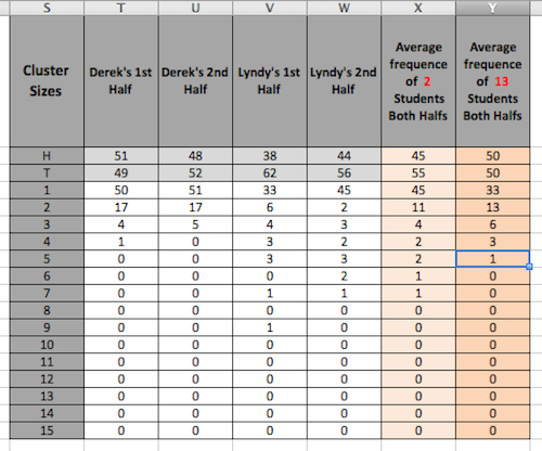
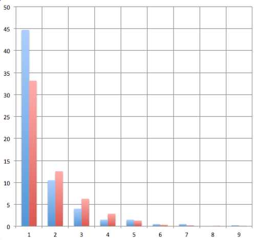
As a side note: the default of the criteria is really "=", so if we are testing for values that ar equal we can omit the operator. I.e., we only need to type: =COUNTIF($I$3:$I$102, S4) . - Frequence Histogram (Learning Charts in Excel). For this question, you will need to show the result of one seqquence of 100 toses, the result of the 'average' of 20 sequences of 100 tosses. The below chart in column X shows the average frequence of 4 sequences of 100 tosses (column T, U, V and W are averaged, and in Y the averate fo 26 sequences (these columns are not shown).
The histogram is shown below:
End result:
Here is a tutorial on drawin bar graphs: http://www.ncsu.edu/labwrite/res/gt/gt-bar-home.html . This tutorial also introduces the FREQUENCY() function so that a 'bar' in the histogram can represent a rnage of values instead of a single value (in our example a specific length of a string.
Grade 50 points total
5 points for emailing your excel file
10 points for
question 2
15 points for question 3
10 points for question 4
10 points for question 5